Jed Homer

Astrophysicist working in Deep Learning. PhD student in Cosmology and Machine Learning with IMPRS at the Observatory of LMU, Munich and the Munich Center for Machine Learning.
Home | Research & Projects | Photographs & Drawings | Other
22/11/2025
Density deconvolution with flow matching
I implemented a the very nice density deconvolution algorithm in Learning Diffusion Priors from Observations by Expectation Maximization (Rozet++24) using a rectified flow model (instead of their variance-exploding-SDE diffusion model).
The basic idea is shown in a toy example here
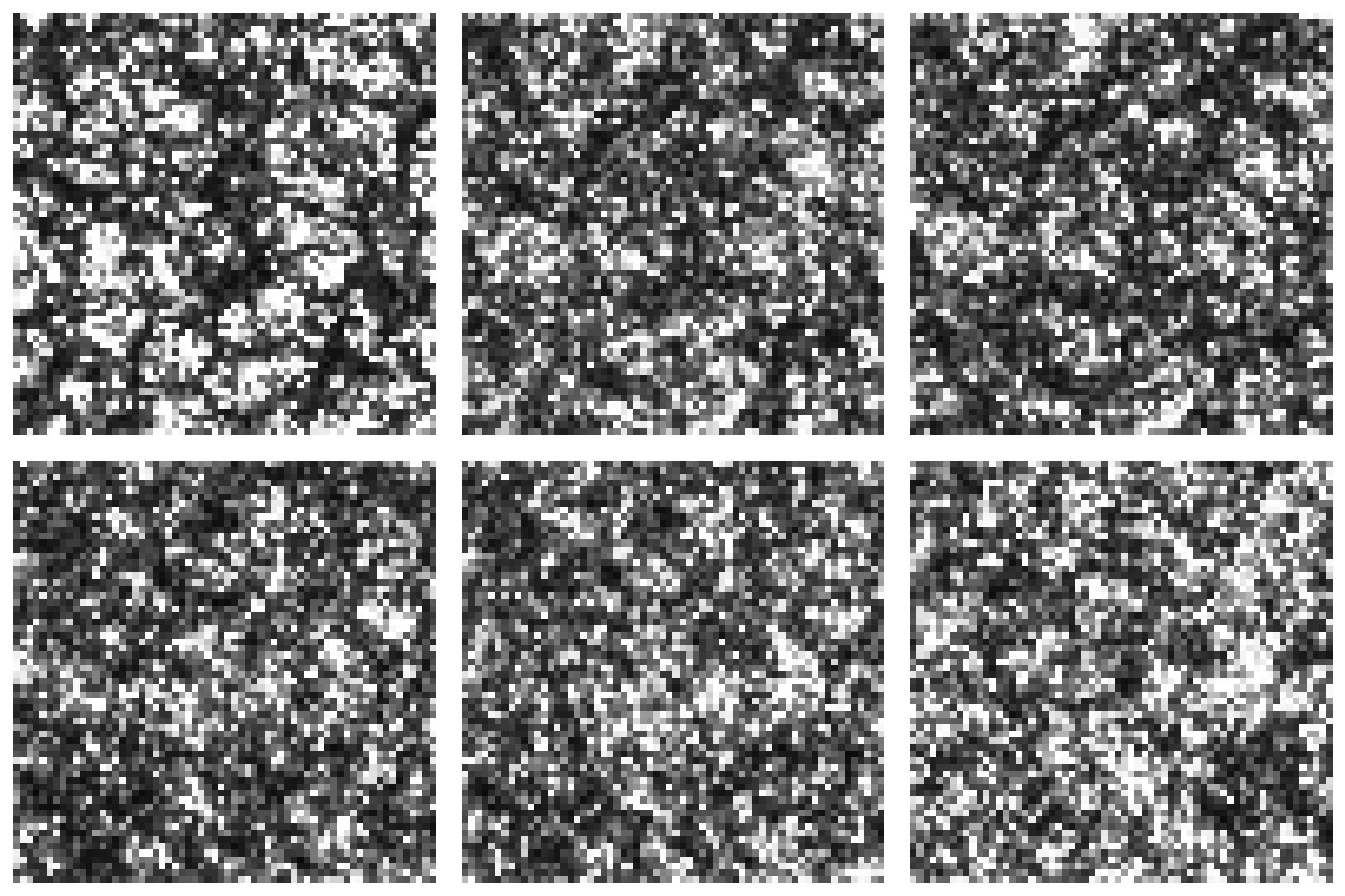
The test case here is on mock galaxy images with varying bulge, ellipiticity and rotation parameters. Top row is what the model deconvolves (and is trained) on and the bottom row are clean samples from the learned, deconvolved, density.
22/11/2025
Random cool jax stuff
Here is a bunch of very useful stuff I didn't know jax did despite being a user for 2 years now.
- Implement host-based operations via https://docs.jax.dev/en/latest/external-callbacks.html even when inside
jit'd operations, - Implement
C++functions insidejaxcodes with Foreign Function Interfaces, Ref: mutable arrays for data plumbing and memory control,- Super useful training cookbook.
11/11/2025
Reconstruction with flow matching
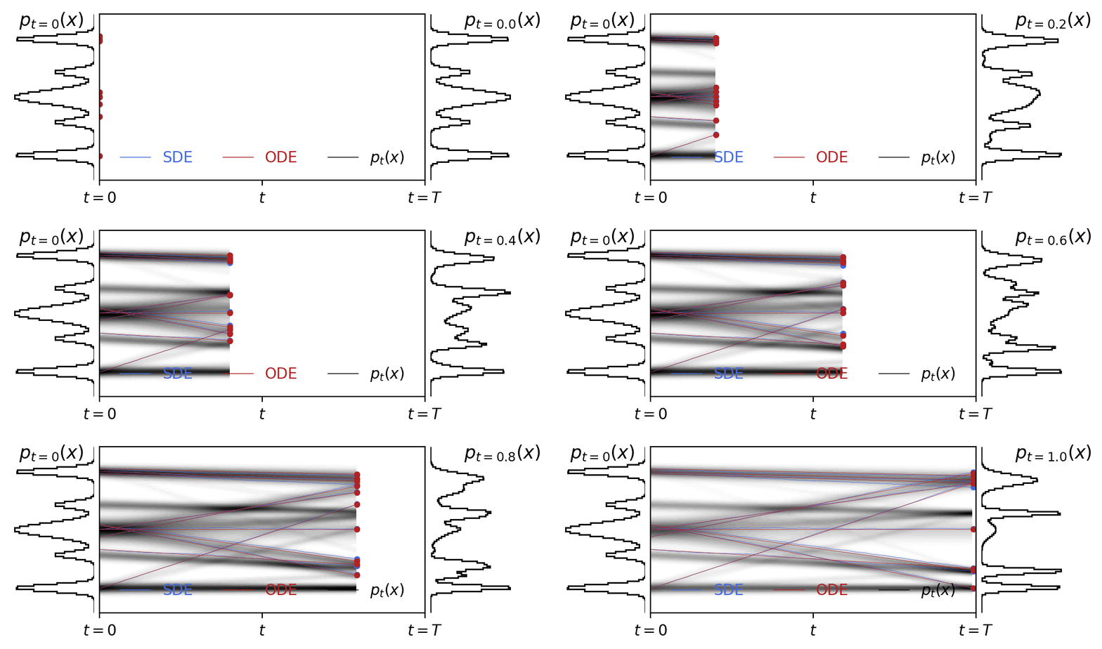
This diagram shows a data distribution (right, blue) reconstructed with samples from a flow matching model. The dataset is mapped back to the prior and reconstructed with the velocity network. As you can see, where you return to in data space is not where you started. This is because of two problems, 1) the ODE solution is numerically imperfect and 2) the neural network approximation error in trying to approximate the ground-truth marginal velocity.
13/08/2025
Stochastic Interpolants
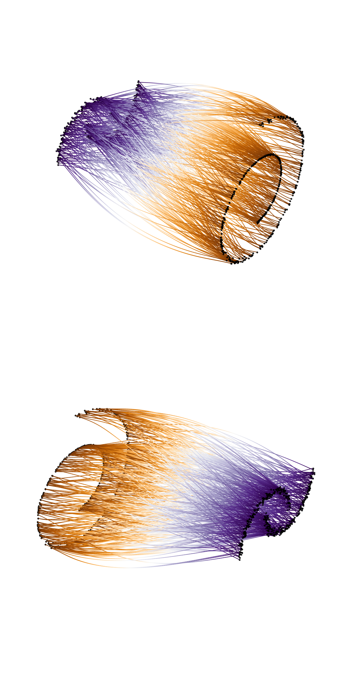
This is an image of a stochastic interpolant mapping from two arbitrary distributions.
I finally took the time to look into this paper: (Albergo++23).
Code is coming soon.
31/07/2025
Rectified Flows
This is an animation of the forward diffusion process associated with a Rectified Flow (Liu++22).
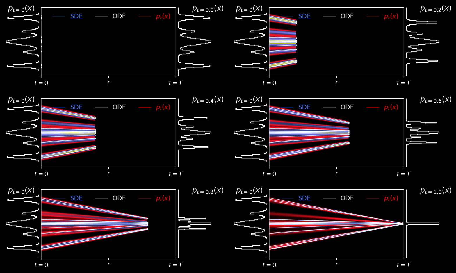
An under appreciated feature of rectified flows is that fitting the velocity field as a function of the diffusion time does not preclude the use of a non-analytic distribution as the prior.
Code is here.
17/07/2025
Bayes & AI Seminar
Slides for a talk I gave today at LMU aimed at MSc students and faculty.
15/07/2025
I wrote a small foundation model
Baryonification with Transfusion: multi-modal diffusion with a unified latent space.
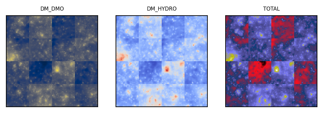
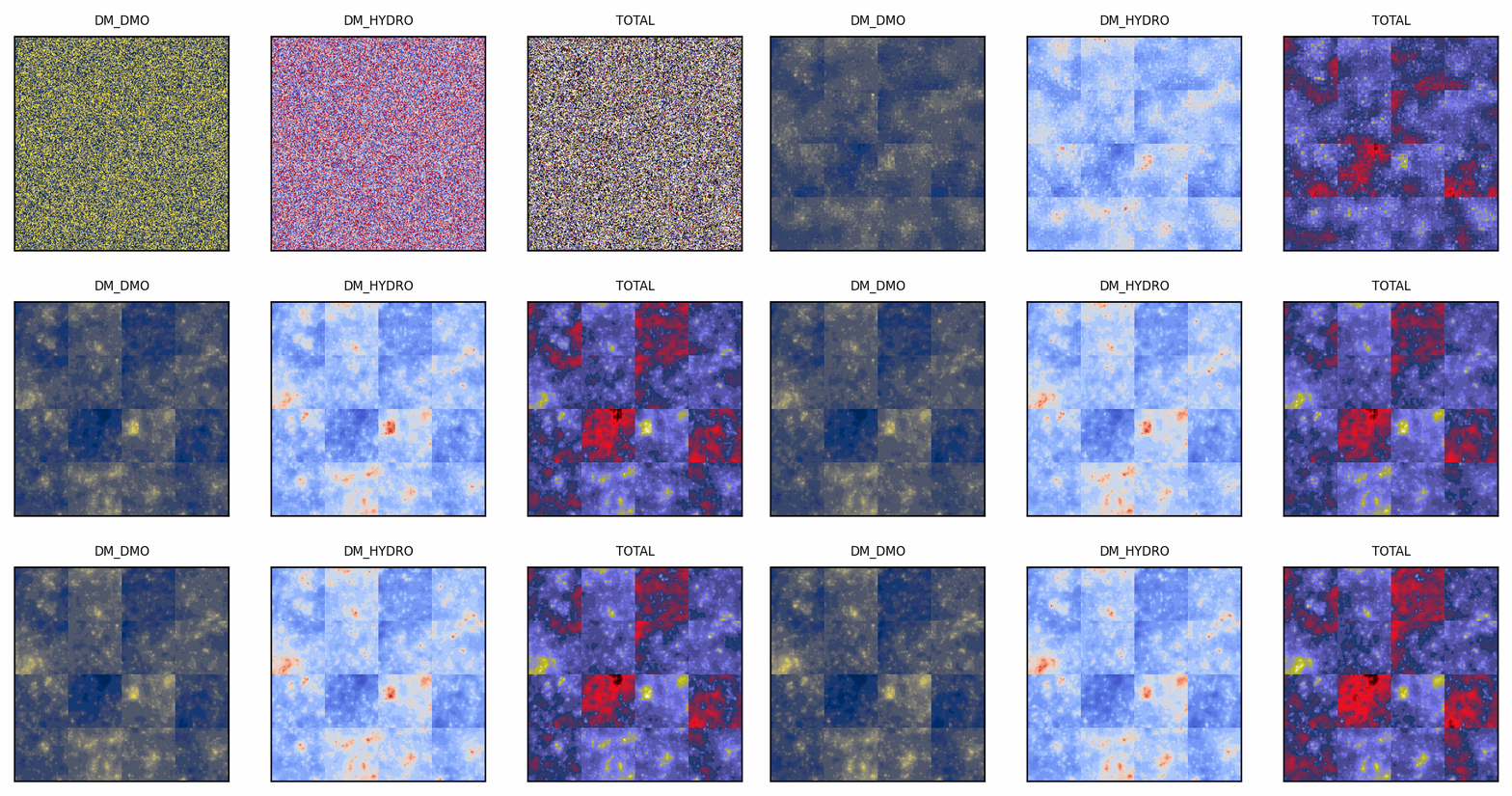
These images are from training a transfusion model for about 30 minutes on 1 A40 GPU as part of a project with Jozef Bucko (ETH) and Tomasz Kacprzak (Swiss Data Science Institute).
That's about 15000 steps with a training set of 10,000 images including 5 "modalities" from the Flamingo simulations. I've used hydro, gas, star, dark matter and "total" (including all physics) maps.
There is a single transformer that "perceives" the different modalities shown below. Each modality is flowed by its own diffusion and time embedding with its own encoder and decoder (note that in this space the transformer attends to sequences comprising every modality).
Here are some samples from the model...
...here are the samples throughout the (incomplete) training...
...and here are some diffusions from the prior to data space...

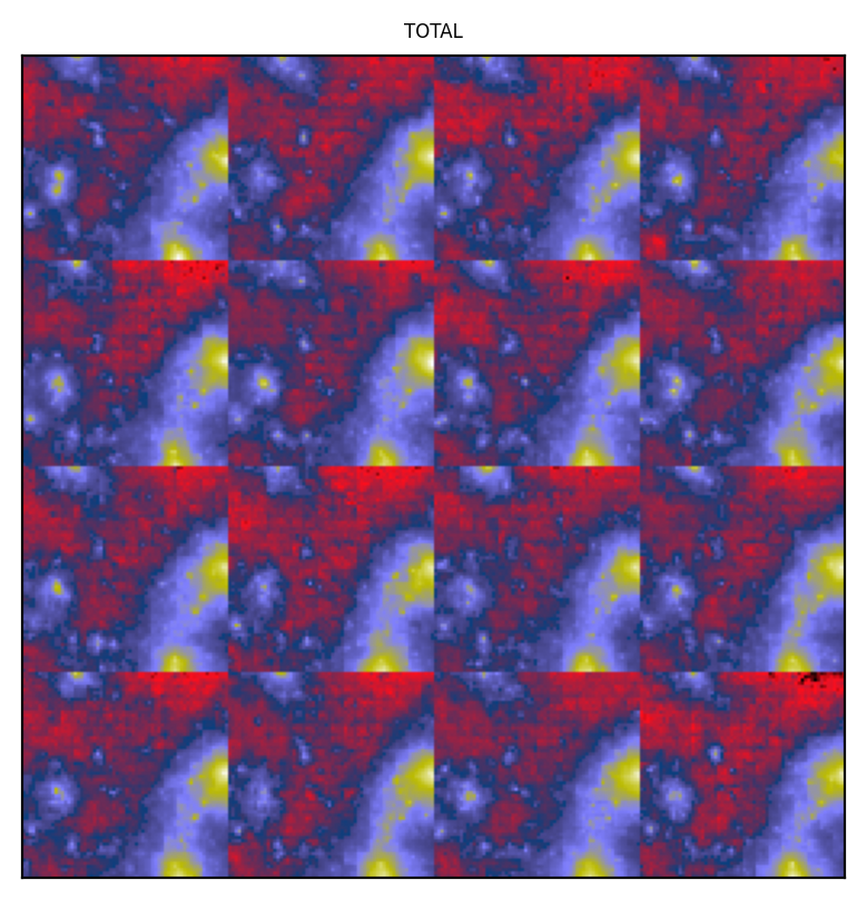
...and last of all, some samples of the "total" maps given a fixed, seed-matched, hydro and dark matter map (there's some token artefacts, but these vanish with more training).
15/03/2025
ClimbGPT
AI for MoonBoards
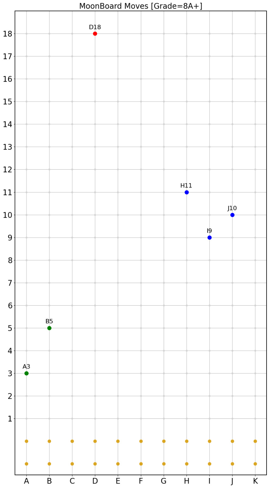
I wrote a small GPT2 to fit to data made from user-defined climbs on the 2016-2019 MoonBoards. The GPT processes a sequence of move coordinates proceeding the grade of the climb. This let's you generate as many holds as you'd like until the end. Unfortunately there isn't enough data from benchmarked climbs. Here is a climb generated by the GPT model given the grade 8a+
28/02/2025
Transfusion
A Realistic Candidate for Foundation Models in Physics
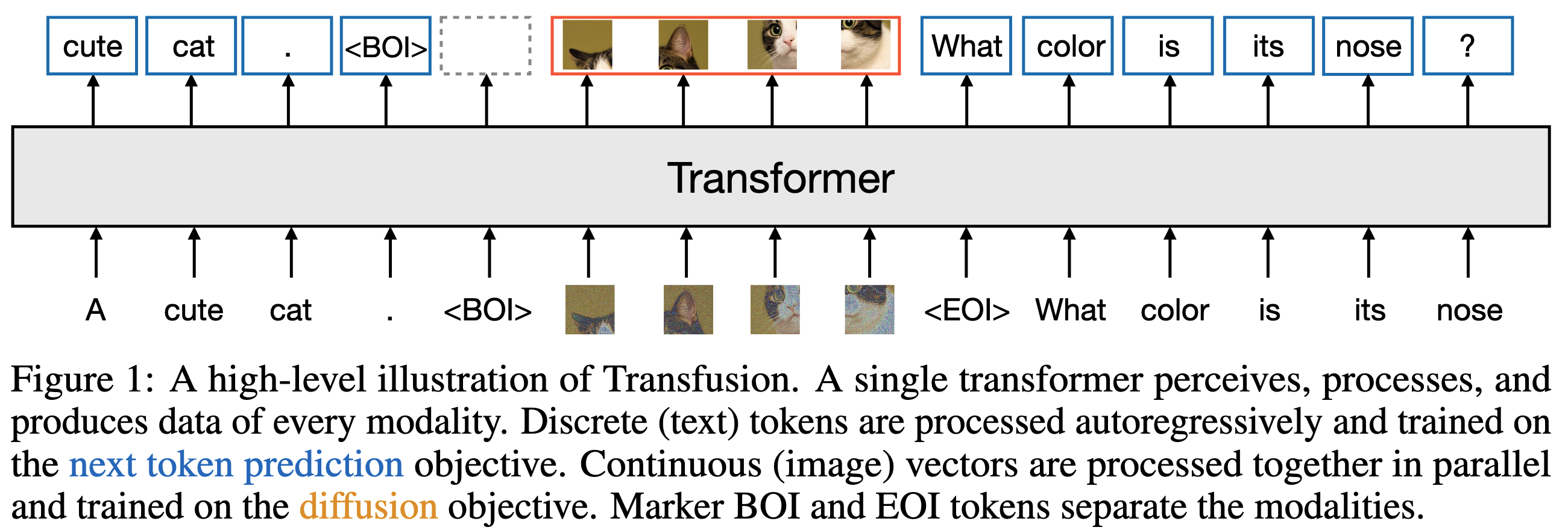
Transfusion is a new algorithm from Meta AI that proposes a very elegant solution to fitting multi-modal generative models without pretraining (excluding the classic VQVAE modules common to foundation models of this kind).
The idea is to use one very large transformer model to process multi-modal dictionaries of tokens from images, text and whatever else.
They use a joint (slightly worrying joint-objective but it seems to work nicely) which obtains some SOTA-level results in image generation and text tasks.
Note that the transformer model is simultaneously trained, token-wise, on denoising diffusion and next-token prediction.
Personally I think this is one of the simplest, most-elegant and valuable solutions in the space of multi-modal generative models - you can explore all the separate conditionings of your point PDF for free, you don't actually need the VQVAE and the objective doesn't exclude normalising flows (not simple though!).
The conditional sampling with this model would be done by denoising, for example, half the tokens in a sequence corresponding to one modality whilst the transformer processes the whole sequence (that may contain other conditioning modalities).
14/02/2025
Talk at Origins Excellence Cluster Data Science Lab
Slides for a talk I gave today at ODSL in Munich.
13/02/2025
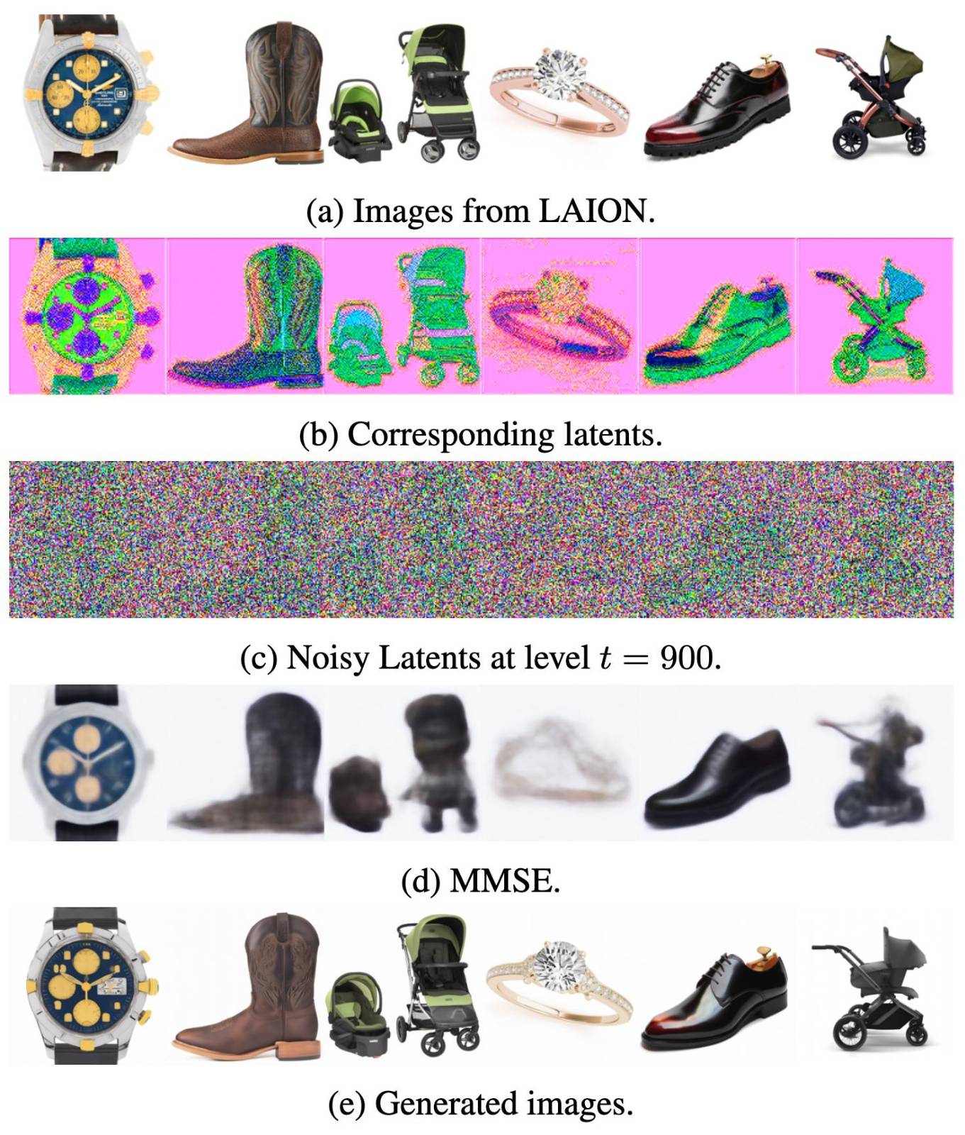
Diffusion models for latents from noisy observations
Consistent Diffusion Meets Tweedie:Training Exact Ambient Diffusion Models with Noisy Data.
Very nice paper by researchers at TU Austin / MIT about training generative models to recover a model for latent variables that are only observed via a corruption process (e.g. no clean training data).
This is a very novel method that depends on a subtle application of Tweedie's formula. In contrast to the paper I posted below, this doesn't require a two-step iteration process (though the model is sampled during training for the consistency of the diffusion model at noise levels below that of the observed data).
The loss has two terms for noise that is above or below the variance of the implicit noise in the data (it's not a potentially risqué double objective like e.g. a VAE).
The consistency term requires mid-training-step sampling - this is reminiscent of the consistency flow matching method from the Ermon group.
One limitation I see here is that the work considers uniform diffusion (e.g. each marginal has a isotropic covariance) meaning that correlated noise corruptions on the data cannot be denoised accurately.
Here's a figure showing the method on a fine tuned large-scale generative model.
11/02/2025
Talk at Max-Planck-Institut für Astrophysik
Slides for a talk I gave today at MPA.
23/01/2025
The latent data-likelihood
Learning Diffusion Priors from Observations by Expectation Maximization (Rozet++24)
Excellent paper about fitting diffusion models to the likelihood of a set of data that is corrupted by a linear operator (e.g. masking and Gaussian noise).
This is a step above the literature on this topic in my opinion: provably fitting the underlying distribution without hacky extra training or modelling assumptions on the corruption proccess - these are compromises that are typical in the 'inverse problem' literature (c.f. diffusion posterior sampling). It should be noted - noiseless/uncorrupted samples are not required to fit the diffusion prior.
I've implemented this myself on a toy problem and it's probably got some bugs in it. They recommend the EDM diffusion method and use a special posterior sampling for the latents (e.g. the uncorrupted data). This involves approximating the covariance of the diffusion kernel as a function of the diffusion time.
I'll come back to my implementation and add flow matching to help with convergence. The expectation-maximisation (EM) step is supposed to assign high marginal likelihood to the observed data with a generative model for the signal as a prior (assuming a known form for the likelihood of the data give the signal!). Whilst iterative two-step methods aren't usually that attractive, I think the use of the EM algorithm is very clearly motivated (and much better than the other options!). This is computationally quite expensive, it should be noted.
In this figure from the paper, you're seeing a images (bottom row) corrupted to a set of data (top row). A sample from the posterior (using the diffusion prior) as a function of the number of EM iterations in each row. This shows the diffusion prior is an effective model for describing the underlying latent likelihood!
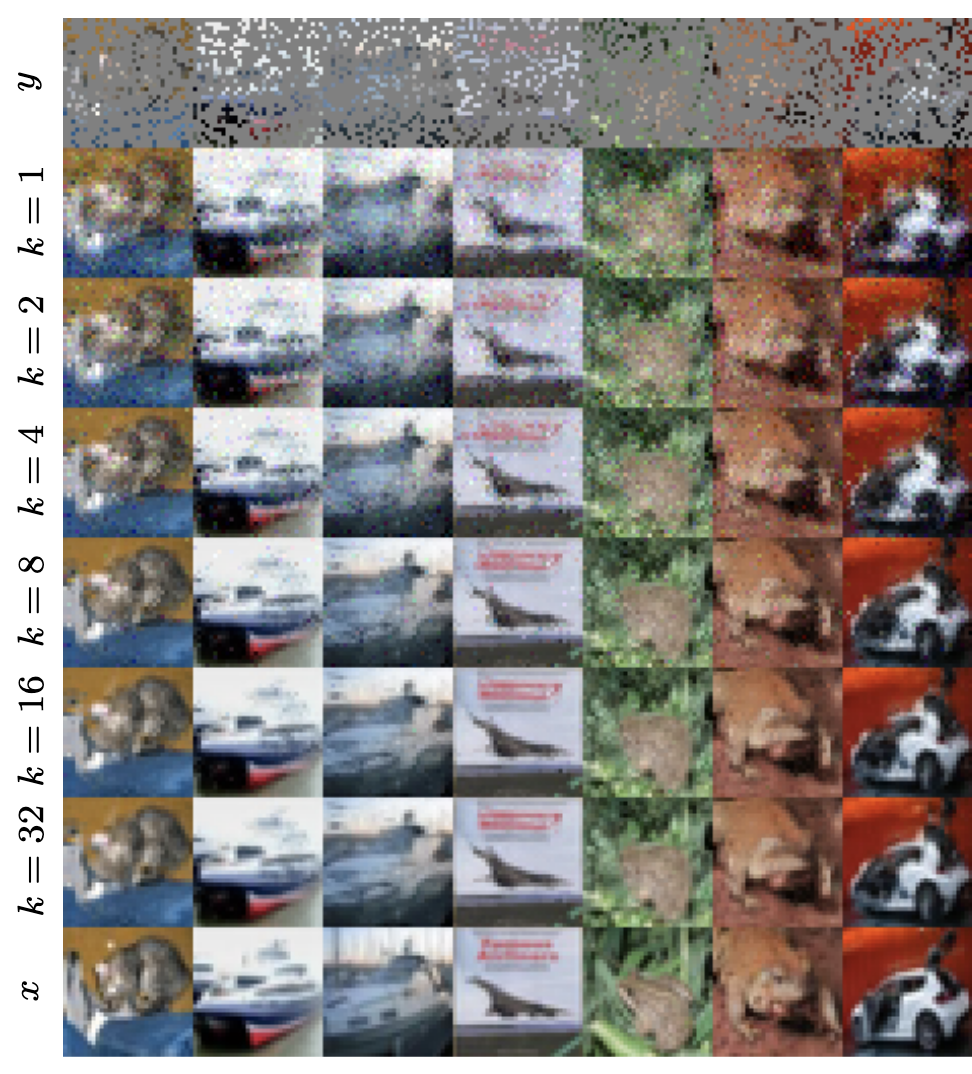
Image Credit: from the original paper.
22/01/2025
Losses for generative models
A note on the evaluation of generative models (Theis++16)
Interesting short paper about the compromises between choosing different loss functions for training generative models.
Finally a source for the strange assertion "log-likelihood is not associated with sample quality".
I'm not 100% sure where e.g. score-matching would fit in here, but probably in the KLD scheme, since you match the perturbed distributions at each step in the diffusion process.
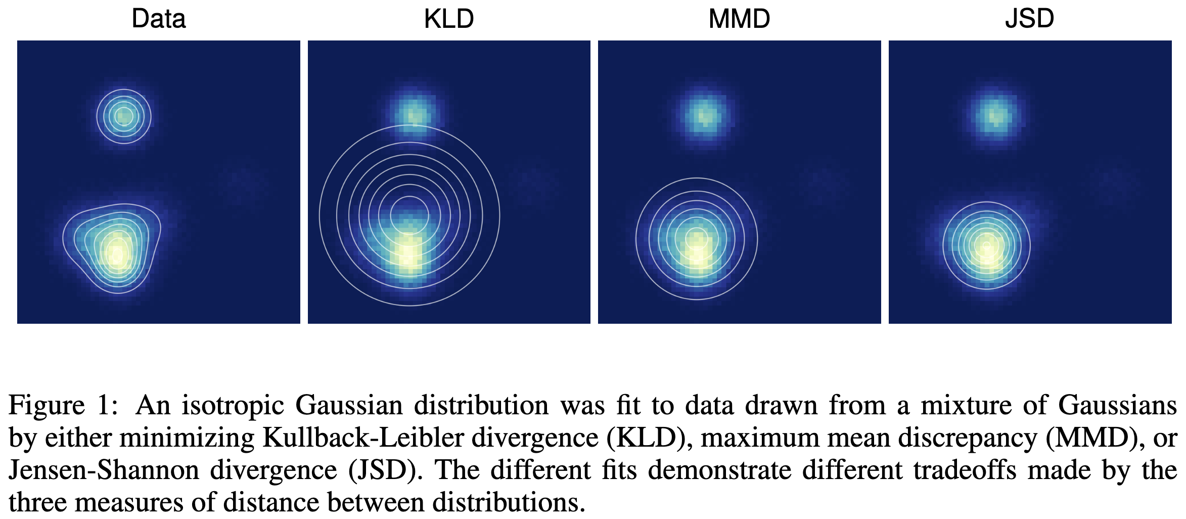
Image Credit: from the original paper.
20/01/2025
Transformer flows
Autoregressive image modelling with transformers and NVP flows
I implemented a recent paper from Apple Machine Learning - Normalizing Flows Are Capable Generative Models.
This was quite a challenge. The paper demonstrates a significant increase in the bits-per-dimension (a.k.a. log-likelihood) of image modelling compared to diffusion and flow matching models of the last five or so years.
The NVP flow model is used for each token (image patch) in a sequence (image); shifting, scaling and permuting the token with the shift and scaling parameters computed by a causal transformer network. In the diagram, $t \in [0, T]$ is the block index and $i\in [0, D]$ is the token index.
The sampling procedure involves the use of key-value caches to autoregressively sample, this is not trivial to implement, particularly in jax. This same technique is used in large language models.
See here for the code.
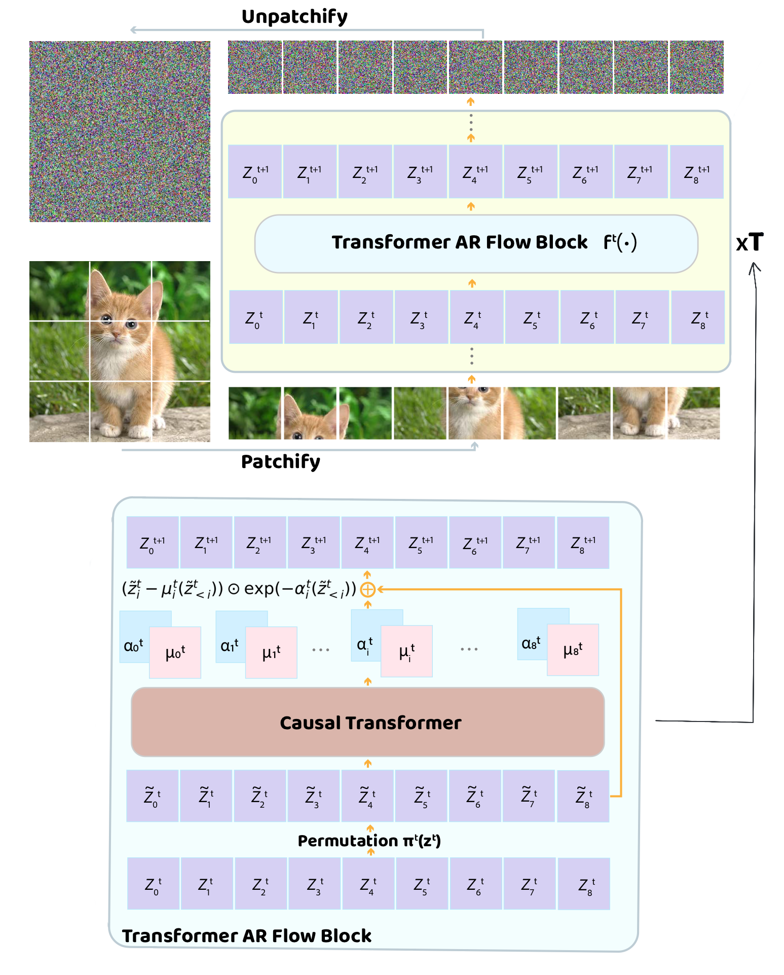
Image Credit: adapted from the original paper.
15/01/2025
sbiax
Density-estimation simulation-based inference in jax
I've released a code for running NPE/NLE-based SBI with normalising flows.
See here.
This package implements Gaussian mixtures, Masked autoregressive flows and continuous flows for now, with fast MCMC-sampling in blackjax.
Use it via
pip install sbiax

See also:
05/04/2023
Probability of the cosmos
I worked with Oliver Friedrich (USM/LMU) as a teaching assistant for his course "The Probability of the Cosmos - Classical, Quantum, Bayesian", a masters level course in probability, cosmology and quantum theory at LMU. Honestly he wrote 99.9% of the notes but I contributed a small section (and plan to add a bit more) about machine learning.
I think this is an exceptional course with a lot of unique information. Like most great teaching material concepts are not simply stated and tend to be backed up with simple objective diagrams.
See the lecture notes here.
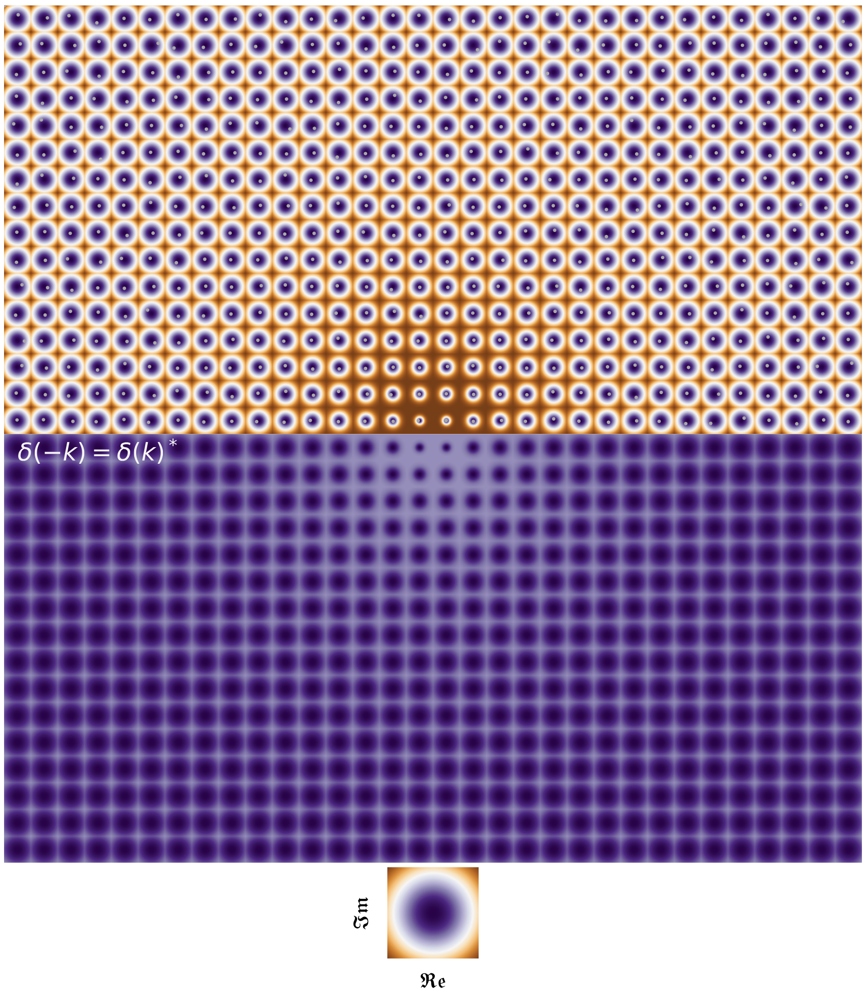
Image Credit: I made this diagram for the lecture notes.
20/10/2022
Painting of the day
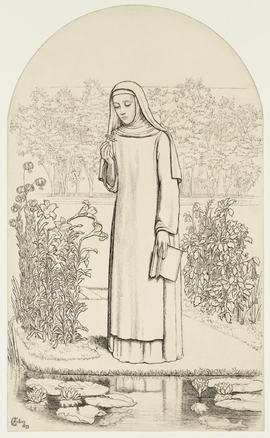
Convent Thoughts - Charles Allston Collins
(This is the prepatory drawing of the painting)
10/10/2022
Bayesian normalizing flows
Clear and interesting paper that gives a lot to think about...
19/09/2022
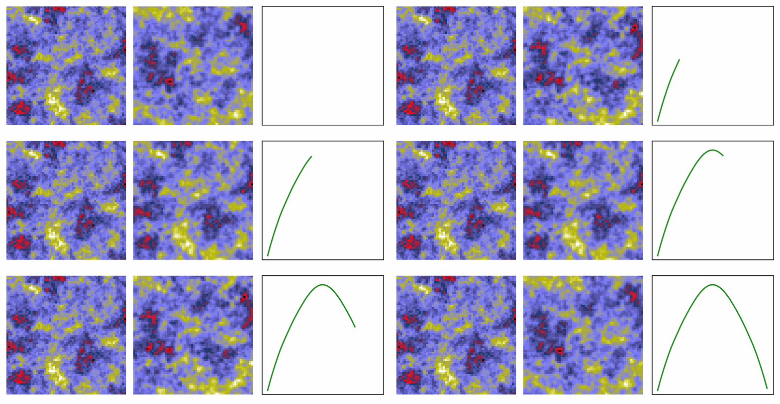
Generative models for inference
Find the target given a noisy observation.
Very excited by the idea of ML in the wilderness of actual observations, as opposed to simulations.
On the left is a noisy realisation and on the right a generative model does its magic!
16/09/2022
"Scissors cutting grass"
Having a go with the open-source Stable Diffusion code.

Image Credit: Source of randomness / latent space :)
01/07/2021
SWAGAN emulating density maps
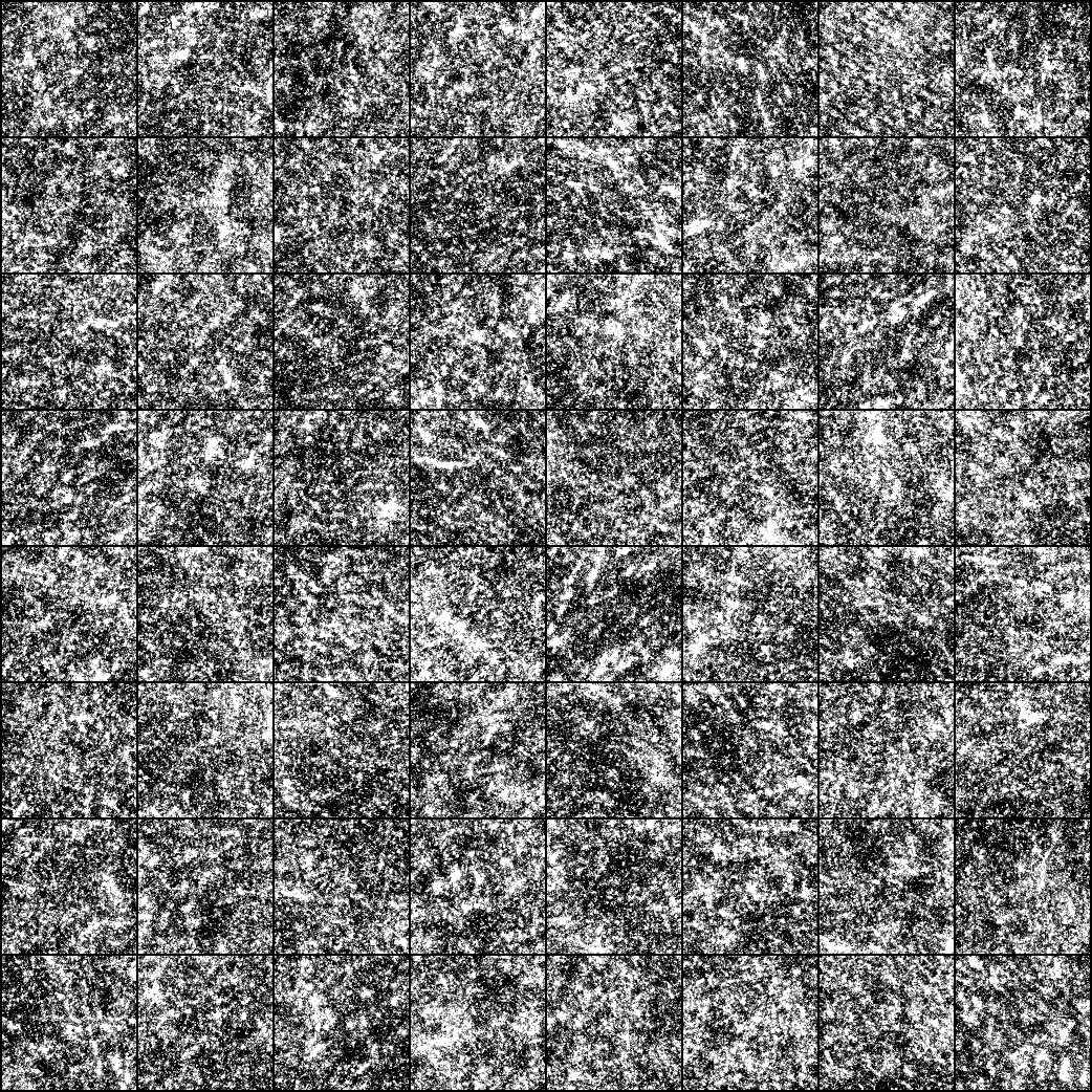
Working on using SWAGAN to generate N-body maps as you will have seen on here before. The results are VERY fast and look great. The quality of the high frequency content is high.
15/06/21
Dreaming in Big Sleep
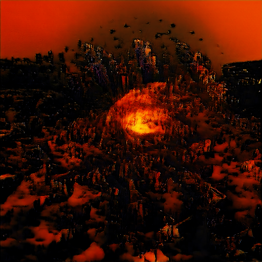
I found a great repository that uses OpenAI's CLIP and DeepMind's BigGAN to create a generative model that can translate sentences into images... very impressive stuff.
This is the result of the sentence "The End of the World"
12/05/21
Physics, ML and Information theory
I'm reading a fascinating book Deep Learning and Physics - Tanaka, Tomiya, Hashimoto (2021) that motivates the use of machine learning in physics by defining the basic instruments of ML from a physics perspective. The Hamiltonian is a central aspect for defining neural networks in a physical way.
The book makes a fascinating point by highlighting that much of modern physics research is in many-body systems - the idea that 'more is different' is central here and shows that statistical mechanics is heavily involved.
Interesting Links:
(image source: second link above)
09/05/21
AI Poincare: Machine Learning Conservation Laws
Physics informed machine learning at its finest (I've not fully read this but you know when you know!).
AI Poincar´e: Machine Learning Conservation Laws from Trajectories
15/04/21
On the use of Neural Networks in physics
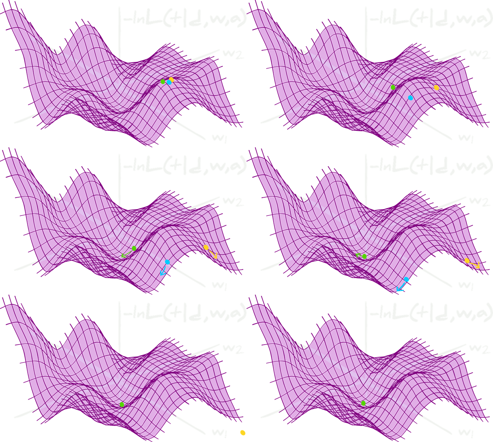
Very interesting discussion on the use and mis-use of neural networks in the physical sciences.
A good point on the merits of Bayesian machine learning.
(image source: The Aquila Consortium)
12/04/21
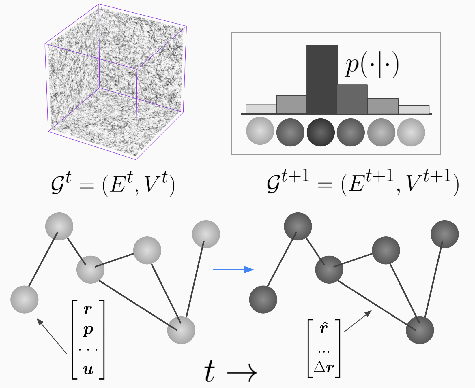
Graph GANs
See this paper here for an implementation of GANs on graph structures.
The paper demonstrates the algorithm on graphs of MNIST superpixel images and high energy jets from particle physics data.
05/04/21
Painting of the day
Jan Beutener - Aardapples (1969)
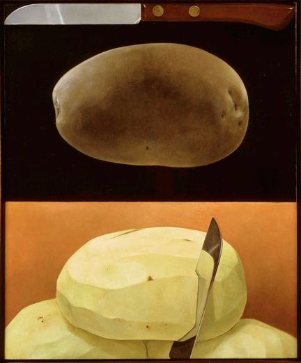
(image source: The Stedelijk, Amsterdam)
27/03/21
Marcus Hutter
Prof. Marcus Hutter has a lot of fascinating work. See here for great references in to artificial intelligence, AGI and more.
This paper is very interesting - Learning curve theory - Hutter (2021) exploring the behaviours of network capacity and data set sizes.
25/02/21
Painting of the day
Yves Tanguy - Imaginary Numbers
I've always wondered if the artist here had any knowledge or imaginary numbers to motivate this painting.
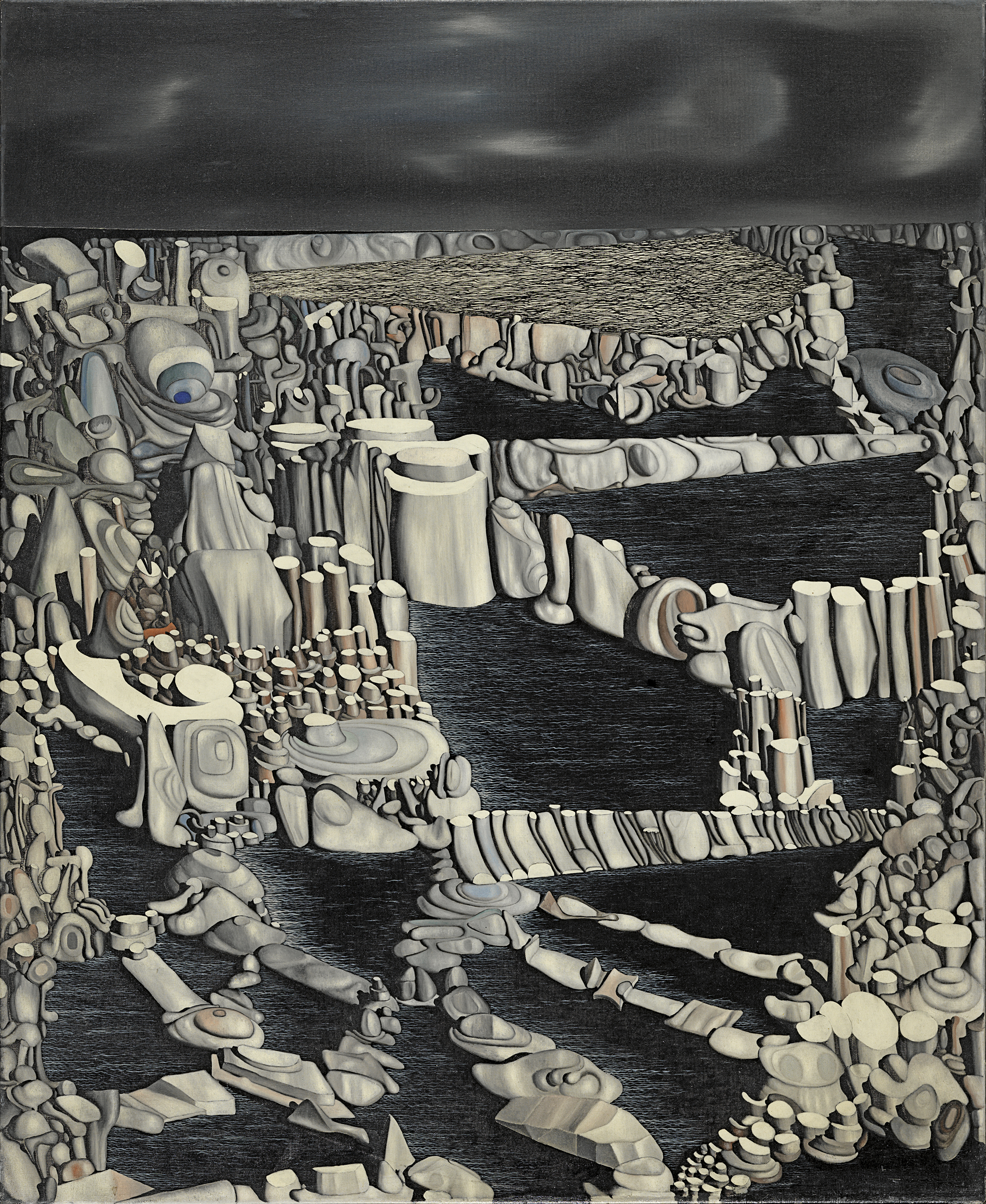
(image source: Museo Thyssen-Bornemisza, Madrid.)
17/02/21
The Moon Landing Code
See this link here for the original Assembly scripts for landing the Apollo-11 Mission on the moon. Unbelievable stuff.
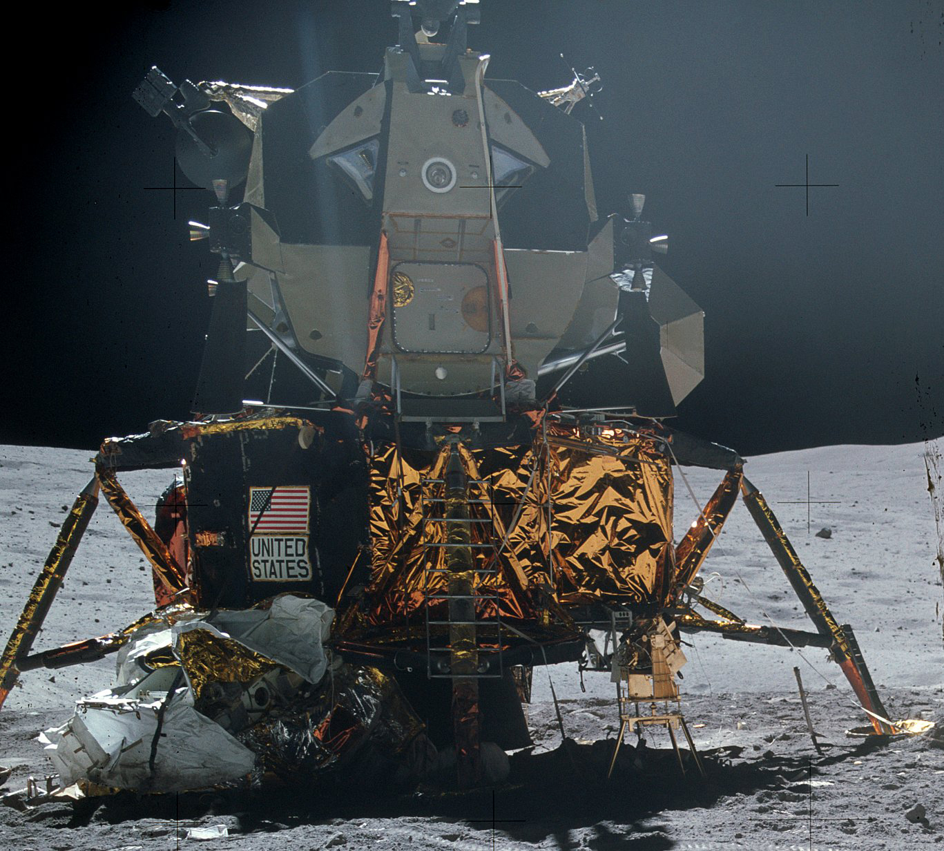
(Image from here)
16/02/21
IMPRS / LMU
I have just received an offer for a PhD from the IMPRS provision, based at the Ludwig-Maximilians-Universität, München.
This is a position in Cosmology in Artificial Intelligence working with Prof. Dr. Daniel Grün.
woooooooooooooooooooooooooooooooo!

(Image from here)
07/02/21
Essential Reading
Daniel Baumann - TASI Lectures on Inflation
See here.

(Image from linked document)
04/02/21
Generative Models Tutorial
I've written a tutorial on Generative Adversarial Networks (GANs) in PyTorch.
You can see the material here.
The idea is to demonstrate generative models with a simple example that balances tangibility and complexity.
The generator learns points that are sampled from a spherical shell.
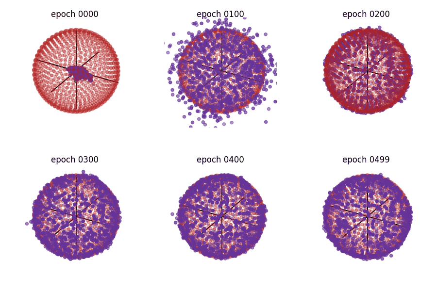
I like PyTorch because its functionality is closer to a differentiable programming language.
I will extend my tutorials to Normalising Flows, VAEs and any other interesting generative models.
(Diagrams are author's own)
03/02/21
Simulating Physics with Graph NNs
Essential modern machine learning work into simulating physics with graph neural networks. I'd like to see this done for cosmological simulations.
I think machine learning techniques would be perfect for upscaling very high resolution smaller simulations. The processes are also very closely linked, especially with the advent of differentiable programming becoming the norm.

(image from original paper)
03/02/21
Painting of the day
Leonardo Da Vinci - Virgin of the Rocks (1483-86)
There are two versions of this painting in existence. This is interesting because Da Vinci tended not to make many pictures, or even finish them.
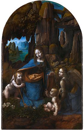
(image source: National Gallery, London)
19/01/21
Randomly wired neural networks
The paper Exploring Randomly Wired Neural Networks for Image Recognition explores the limits of the canonical neural network architecture. Their stochastic network generator creates randomly connected graphs that are able to compete with ResNet-50 for the classification of images.
This is interesting as it could point to a theory for designing architectures based on inductive biases. I imagine their is a problem-dependent optimum.
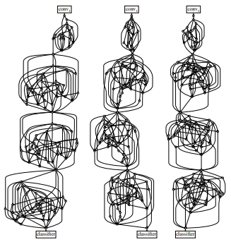
(image from original paper)
17/11/20
DESY and terrestrial black holes
I've been offered a PhD position at DESY, Hamburg.
The project is a mix of generative artificial intelligence, particle physics and simulation inference.
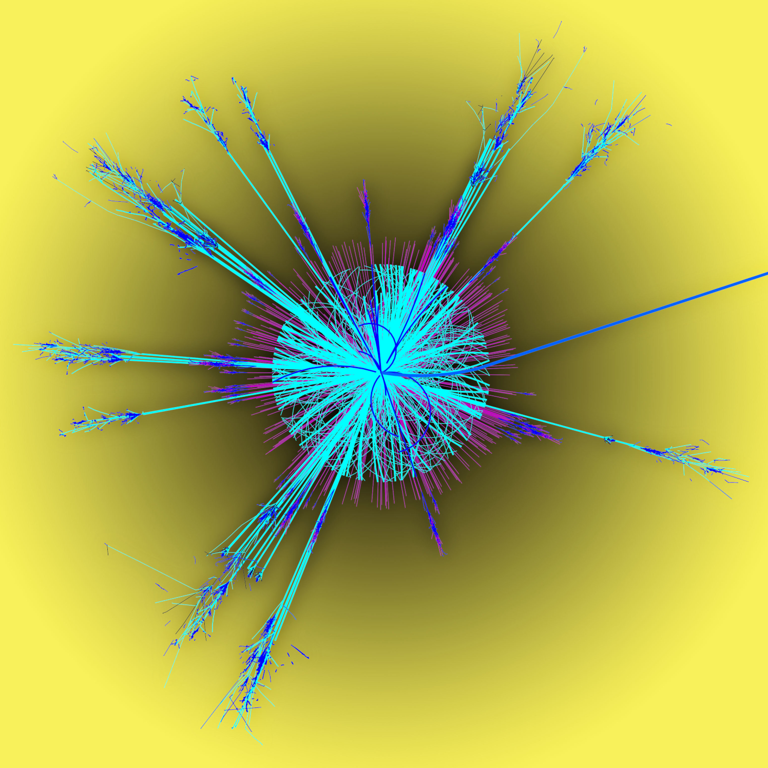
This is a picture from the ATLAS project at CERN of a black hole being formed inside a collider.
17/01/21
Schiehallion
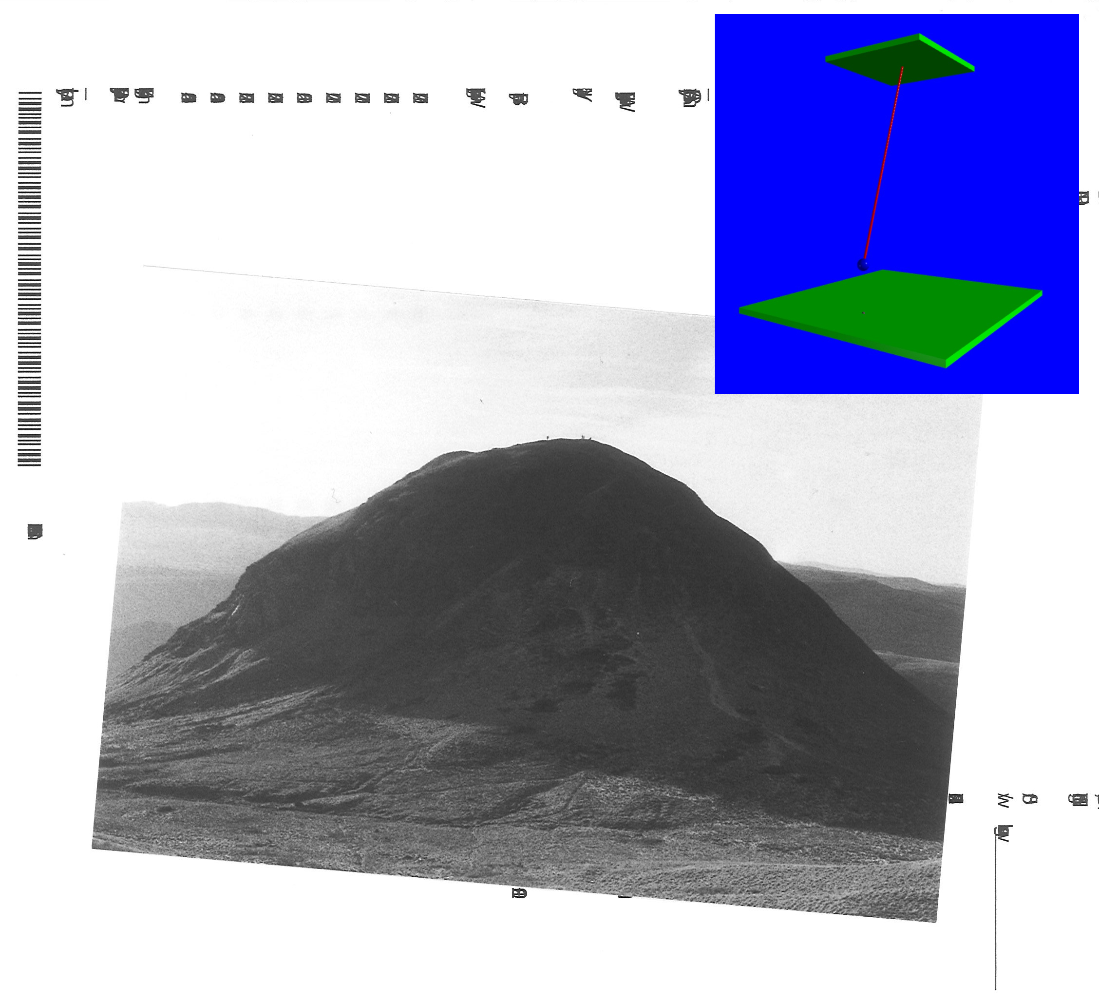
In the summer of 1774 Nevil Maskelyne measured the gravitational deflection of a pendulum from an isolated mass. The isolated mass was the Scottish mountain of Schiehallion in Perthshire.
The angle of deviation away from the radial pull of the Earth's centre of mass was measured by comparing the true zenith against the apparent zenith of the pendulum's string.
13/01/21
Learning physics with neural networks
Lagrangian Neural Networks (Cranmer et al. 2020) are a way to parameterise arbitrary Lagrangians from data linked to coordinates of physical systems (one is not required to have restrictive canonical coordinates).
Previous methods to parameterise physical models (i.e. using position/velocity data to obtain acceleration) do not tend to learn physical symmetries such as energy and momentum. In other words, animating the learnt parameters (position/velocity/acceleration) will not look realistic.
This method learns the conservation laws displayed in the natural phenomena it learns the Lagrangian for. The best part for me is that the gradients of the network are used in calculating the missing parameters.
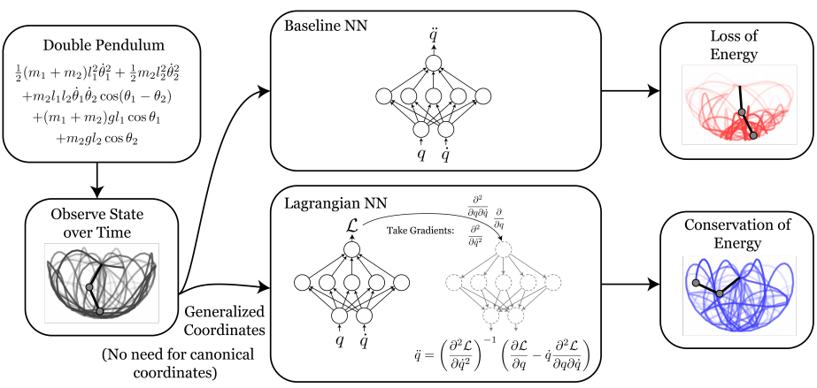
(image from original paper)
07/01/21
Essential Reading
David Tong - Lectures on Theoretical Physics
See here.
21/12/20
Painting of the day
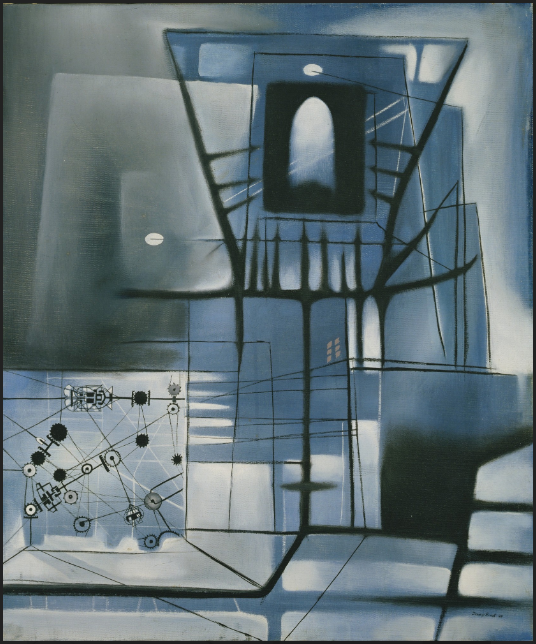
Jimmy Ernst - A Time for Fear (1949)
Sometimes you see a painting like something in the corner of your eye, what you see isn't the same as what caused the appearance, but the image can come back months or even years later.
02/12/20
Artificial redshift evolution
I made a generative model that can interpolate a latent point through redshifts. This means a single cosmic web sample can be evolved over time. The picture below shows the cosmic sample evolving backwards from redshift 0 to redshift 5.28.
A better animation of the process is shown here.
28/10/2020
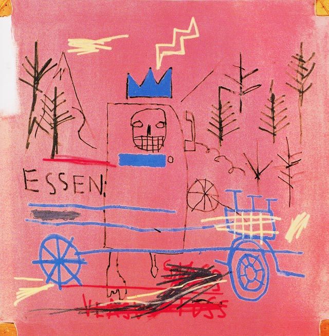
Painting of the day
Jean-Michel Basquiat - Bruno in Appenzel (1982)
26/10/20
Physical Artificial Intelligence
An unbelievable paper here has brought to reality a neural network that you can touch.
Simple architectures are carved into a membrane - the plasticity of the material is the medium in which the progress of learning is recorded... unreal.
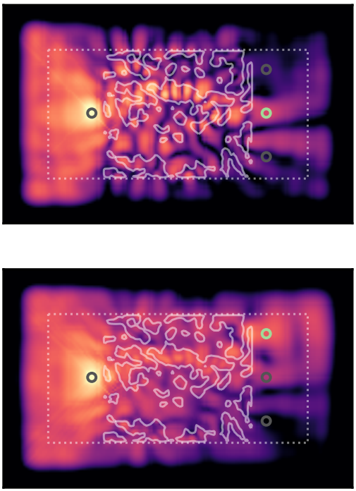
This figure shows contours of the membrane with light wave propagations over the top that allow the communication of nodes to other nodes - the "forward pass" as is commonly known.
21/08/20
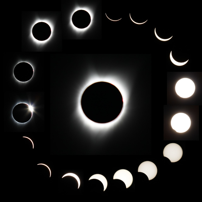
Solar eclipse, Aug. 21 2017
On this day three years ago...
16/08/2020
Painting of the day
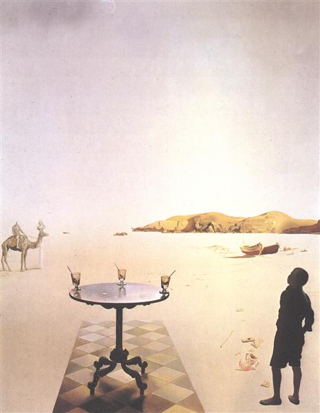
Salvador Dali - Sun Table (1936)
12/08/2020
Quantum CNN
Note to self:
Read this - Quantum Convolutional Neural Network.
04/08/2020
The Fourier Transform.
I think the Fourier transform (FT) is easily one of the most fascinating things I have ever come across. I've been using it recently with my generative models. It might be a simpler/faster/more-elegant way to reproduce the finer structure in the cube-samples of cosmic web.
Here is a picture of the 3D-FFT of three redshift zero cube samples. The first row are the original samples, the second row shows the FT of these samples and the last row is the inverse FT of the second row.
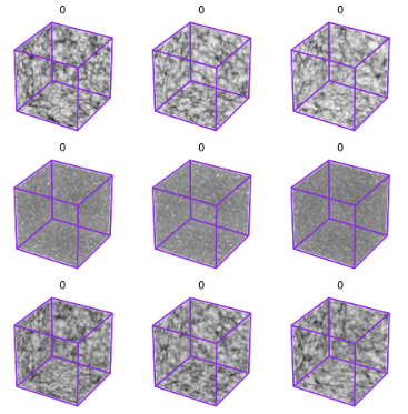
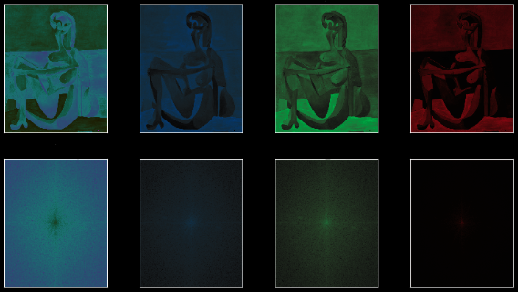
The idea that no information is lost, because the Fourier transform is bijective, is crucial. I can't say I fully understand the transformation but I am fascinated that an orthogonal basis, as a set of independent objects, can represent so many different objects is incredible. I will write more about this in the future.
For now, here is a picture of the FFT of Picasso's 'Seated Bather' (1930).
27|07|2020
Engineering Generative Adversarial Networks (GANs).
It is well known that GANs are very hard to train. I don't like the idea of it being closer to alchemy than science - these methods are supposed to generalise. I feel like sometimes I am over-complicating the beautiful original implementation (Goodfellow et al. 2014).
I'm interested in creating an application to visualise the complications in designing the discriminator and generator models. The problem mainly stems from the constantly changing high-dimensional space the losses for each model are calculated in.
I think looking at the individual layers (the trainable ones in particular) and calculating a metric on their products could point to which part of the models are causing the most problems over training. This could be done in-training and without compiling a complex model of all the outputs of each layer.
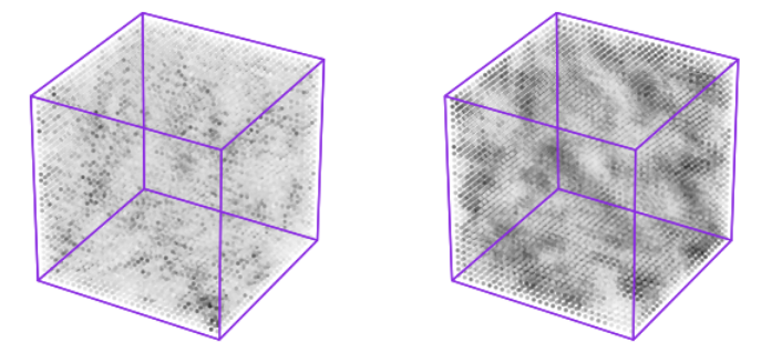
I've written something to look into each layer of the generator and discriminator models. I'm really amazed by what you can see from it. Unforunately, plotting all the feature maps would melt the GPU I use, so here are just two activations from the discriminator:
26|07|2020
Reinforcement learning in Keras.
I'm a huge fan of Tensorflow and the Keras API. It's incredible how tangible modern science has become. In part this is through the openess of the research community in artificial intelligence.
The year is 2020 and you can now reproduce arguably the most advanced machine agent ever created on your own computer. See here for a guide to implementing DeepMind's Atari Agent.
It's worth noting here that the code below from the link above is the 'sensory' faculty of the agent.
def create_q_model():
    # Network defined by the Deepmind paper
    inputs = Input(shape=(84, 84, 4,))

    # Convolutions on the frames on the screen
    layer1 = Conv2D(32, 8, strides=4,
                    activation="relu")(inputs)
    layer2 = Conv2D(64, 4, strides=2,
                    activation="relu")(layer1)
    layer3 = Conv2D(64, 3, strides=1,
                    activation="relu")(layer2)

    layer4 = Flatten()(layer3)

    layer5 = Dense(512,
                   activation="relu")(layer4)
    action = Dense(num_actions,
                   activation="linear")(layer5)

    return Model(inputs=inputs, outputs=action)
Essentially, this model has only the pixels (i.e. the screen) to learn from. These layers initiate a hierarchy of information that is distilled through repeated experience of the Atari games.
24|07|2020
Painting of the day.
Jacopo Pontormo - Visitation (1528–1529)
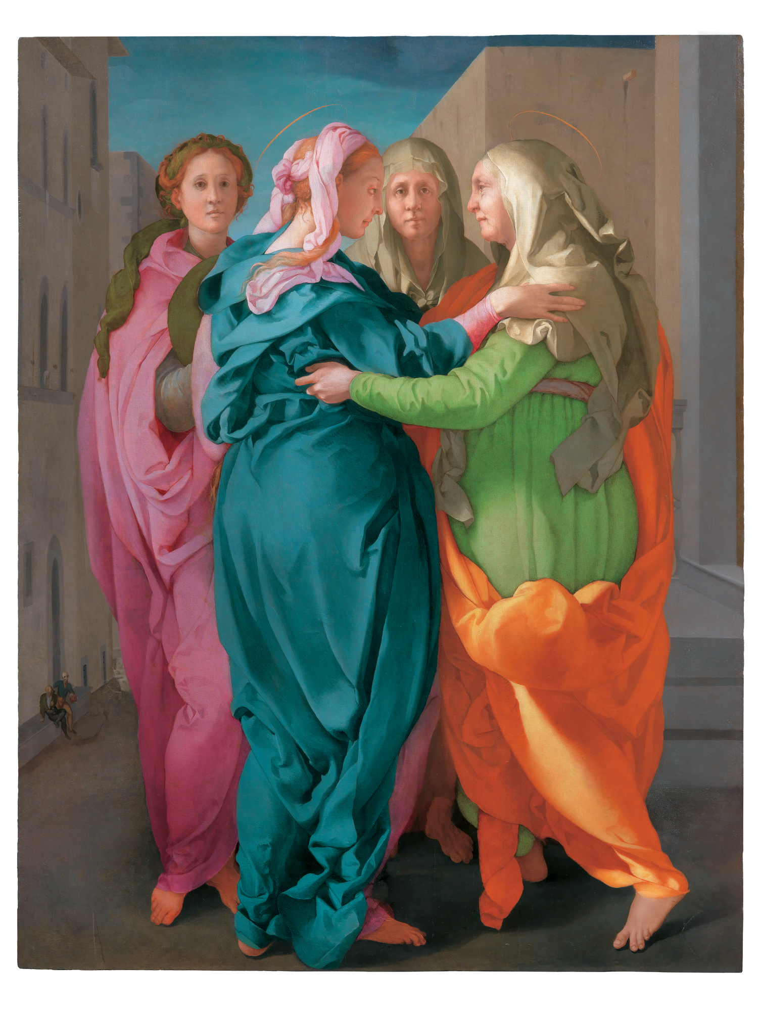 I was lucky to see this a few years ago in the Uffizi Gallery, Florence. It is usually kept in a rural village. As with all paintings in a virtual format, the colours aren't quite right.
A special kind of 'luminosity' is obtained by layering many thin layers of paint. This works well for warming or cooling shadows. Raphael used this technique frequently.
24|07|2020
Cosmological simulations.
I'm looking at a different simulation for use as training data with the GAN.
I have been using the Millennium Project (Springel et al. 2005) SAGE catalogs (Croton et al. 2016).
The sparse nature of filaments and voids seems to be problematic for convolutions with fixed kernels. I think balancing the number of pixels against the size of the filaments in each cube is critical for this.
This is a picture of the MultiDark Simulation which I am going to try instead of the Millennium-SAGE volumes.
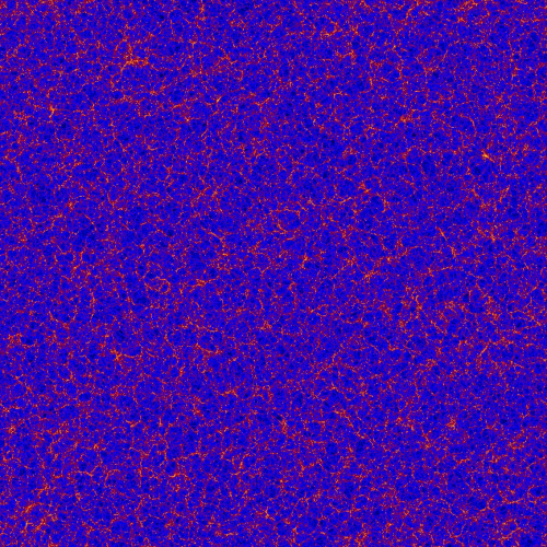
I'm a massive fan of the TAO project. Anyone should be able to access this sort of data even if it is just to look at it for themselves.
23|07|2020
Blueprints.
The initial blueprint for my next painting. The idea changes with each day you look at it and it is best to move quickly with this kind of thing I find.

23|07|2020
An artificial universe.
The first post on my site.
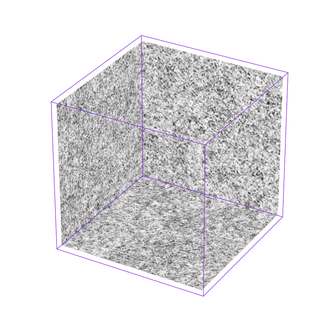
This is a box of galaxies of side length 1440 Mpc / h that was made by piecing together a collection of 1729 cubes created by a Generative Adversarial Network.
